Data Loader: Data Scaling
This page allows you to specify parameters for scaling the actual trace
data. You might need to scale the data when converting to a
different format, or to remove spikes from your data. Scaling
is
also useful when trying to balance all your data to the same relative
amplitudes.
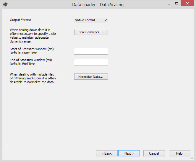
Output
Format:
Specify the format of the output trace data. Normally you
will
leave this as Native Format. You may want to change this
option
to save disk space or when scaling all your data to have the same RMS
value.
- Native
Format:
The
output traces are written in the same format as the input
traces.
The only exception is for IBM floating point data. If the
input
traces are IBM floating point they are written out as IEEE floating
point data. This is the most common option you will select.
- IEEE Float: Write the data as IEEE floating point data. IEEE is the normal format for floating point values on a PC. It has the best dynamic range of all formats.
- IBM Float: Write the data as IBM floating point data. You will not normally choose this option. IBM floating point is slow because it requires data to be converted to the native PC format before being used. You would only choose this option if you intend to use the file in another package that requires IBM floating point data.
- 32 Bit Integer: Write the data as 32 bit integer values. This format is very uncommon and almost never used.
- 16 Bit Integer: Write the data samples as 16 bit integer values. Choose this option to save disk space at the expense of dynamic range.
- 8 Bit Integer: Write the data samples as 8 bit integer values. Choose this option to save disk space with a great loss of dynamic range. This option is not a very common choice.
Scan
Statistics: Click
on the Scan Statistics
button to pop up the Data Statistics
dialog. This will
allow you to scan data for spikes
and
determine
the amplitude distribution of your data.
Start of Statistics Window: Specify the start time or depth used to calculate the peak, average and RMS data statistics. The default value is the start of the data. You may want to specify this value to restrict statistics calculations to your zone of interest, or to clip out spikes in the data for statistics purposes.
End of Statistics Window: Specify the end time or depth used to calculate the peak average and RMS data statistics. The default value is the end of the data. You may want to specify this value to restrict statistics calculations to your zone of interest, or to clip out spikes in the data for statistics purposes.
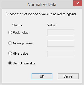
Normalize Data: Pop up the following dialog to allow you to balance the amplitudes of all input files. This step is very useful when loading files from different sources or of different vintages. Typically you will use the RMS statistic to balance your data, although you may also choose the peak or average value. For example, choosing an RMS value of 10,000 will ensure that all loaded files will be scaled to have an RMS value of 10,000. Normalizing data helps to ensure that horizons from different lines have amplitudes that can be easily compared.
Start of Statistics Window: Specify the start time or depth used to calculate the peak, average and RMS data statistics. The default value is the start of the data. You may want to specify this value to restrict statistics calculations to your zone of interest, or to clip out spikes in the data for statistics purposes.
End of Statistics Window: Specify the end time or depth used to calculate the peak average and RMS data statistics. The default value is the end of the data. You may want to specify this value to restrict statistics calculations to your zone of interest, or to clip out spikes in the data for statistics purposes.
Normalize Data: Pop up the following dialog to allow you to balance the amplitudes of all input files. This step is very useful when loading files from different sources or of different vintages. Typically you will use the RMS statistic to balance your data, although you may also choose the peak or average value. For example, choosing an RMS value of 10,000 will ensure that all loaded files will be scaled to have an RMS value of 10,000. Normalizing data helps to ensure that horizons from different lines have amplitudes that can be easily compared.
— MORE INFORMATION

|
Copyright © 2020 | SeisWare International Inc. | All rights reserved |